Principal component analysis(PCA) & Partial least squares regression(PLS)

PCA

A notes from Deep Learning Foundations and Concepts (Christopher M. Bishop, Hugh Bishop)

Principal component analysis, or PCA, is widely used for applications such as dimensionality reduction, lossy data compression, feature extraction, and data visualization. It is also known as the Kosambi–Karhunen–Loeve transform.

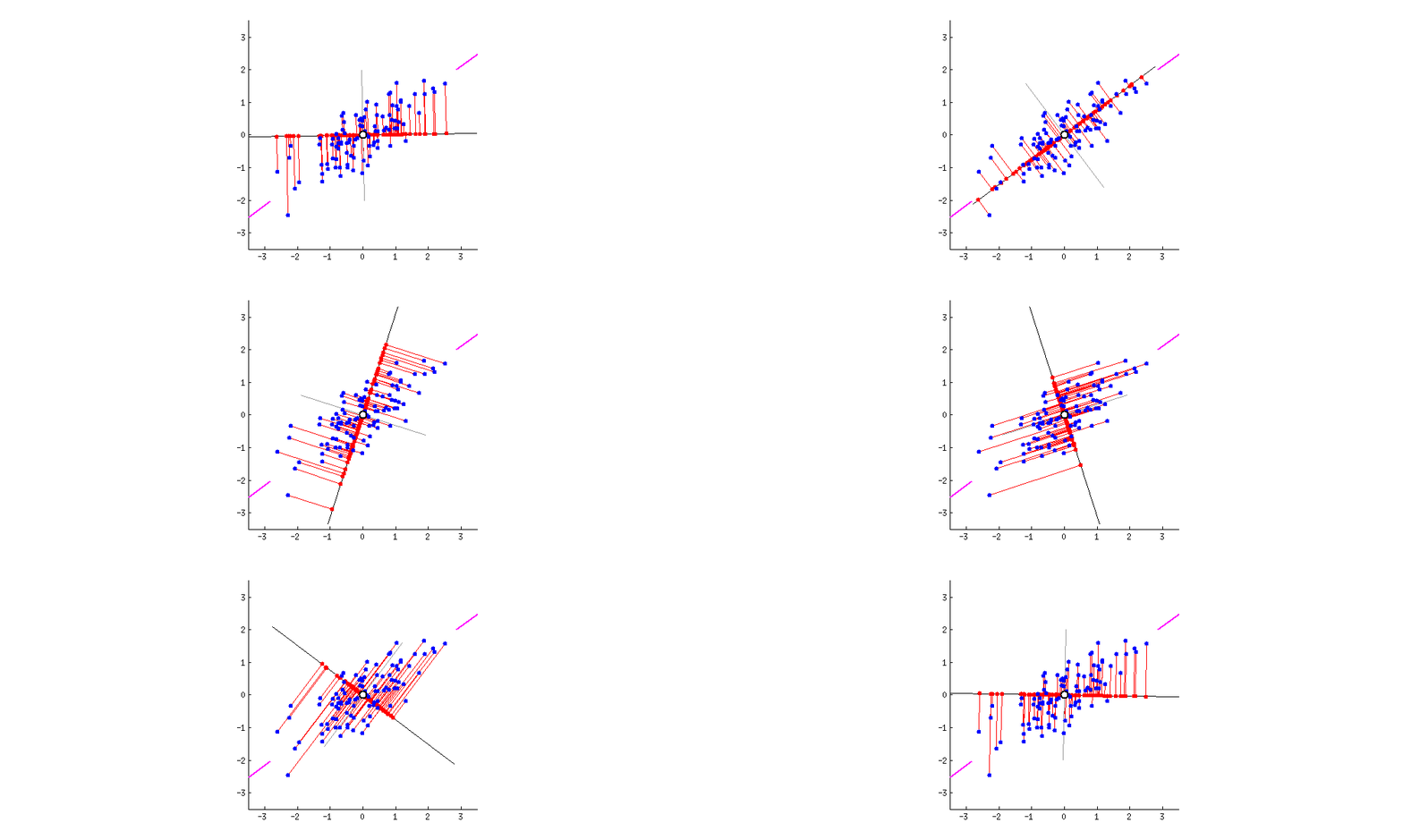
PCA can be defined as the linear proejction that maximizes the variance of the projecrted data, or it can be defined as the linear projection that minimizes the average projection cost(hte mean squared distance between the data points and their projections)

Given a dataset, PCA seeks a space of lower dimensionality(known as principal subspace) that satisfies the definitions above.

Maximum variance formulation

Consider a data set of observations $x_n$ where $n=1,...,N$, and $x_n$ is a variable with dimensionality D.
Our goal is to project the data onto a space having demensionality $M<D$, while maximizing the variance after projected

assume that $M$ is given

When $M=1$, we can define the direction of the space using a $D$-dimensional vector ${\text{u}}_1$, and without loss of generality, we choose ${\text{u}}_1$ that satisfies ${\text{u}}_1^T{\text{u}}_1=1$
then projection of ${\text{x}}_n$ will be ${\text{u}}_1^T{\text{x}}_n$
the mean of the procjected data is ${\text{u}}_1^T\bar{\text{x}}$

$$\overline{\mathbf{x}}=\frac{1}{N}\sum _{n=1}^N{\mathbf{x}}_n$$

the variance will be

$$\frac{1}{N}\sum _{n=1}^N{\left\{{\mathbf{u}}_1^{\mathrm{T}}{\mathbf{x}}_n-{\mathbf{u}}_1^{\mathrm{T}}\overline{\mathbf{x}}\right\}}^2={\mathbf{u}}_1^{\mathrm{T}}\mathbf{S}{\mathbf{u}}_1$$

where $S$ is the data covariance matrix

$$\mathbf{S}=\frac{1}{N}\sum _{n=1}^N({\mathbf{x}}_n-\overline{\mathbf{x}})({\mathbf{x}}_n-\overline{\mathbf{x}}{)}^{\mathrm{T}}.$$

And then maximize the projected variance ${\mathbf{u}}_1^{\mathrm{T}}\mathbf{S}{\mathbf{u}}_1$
To prevent $||u_1||\to \infty$, A appropriate constraint comes from the normalization condition ${\mathbf{u}}_1^{\mathrm{T}}{\mathbf{u}}_1=1$
Introduce a Lagrange multiplier denoted by ${\lambda }_1$
then the formula becomes

$${\mathbf{u}}_1^{\mathrm{T}}\mathbf{S}{\mathbf{u}}_1+{\lambda }_1\left(1-{\mathbf{u}}_1^{\mathrm{T}}{\mathbf{u}}_1\right).$$

Setting the derivative with respect to ${\mathbf{u}}_1$ equal to zero, there is a stationary point when

$${\mathbf{Su}}_1={\lambda }_1{\mathbf{u}}_1,$$

It says that ${\mathbf{u}}_1$ must be an eigenvector of $\mathbf{S}$. If left-multiply by ${\mathbf{u}}_1^{\mathrm{T}}$, and with the condition ${\mathbf{u}}_1^{\mathrm{T}}{\mathbf{u}}_1=1$
the variance will be

$${\mathbf{u}}_1^{\mathrm{T}}\mathbf{S}{\mathbf{u}}_1={\lambda }_1$$

Maximizing the variance becomes choosing the eigonvector ${\mathbf{u}}_1$ that has the largest eigonvalue ${\lambda }_1$. This eigonvector is kown as the first principal component

We can then define additional principal components in an incremental fashion(增量) by choosing each new direction to be that which maximizes the projected variance amongst all possible directions orthogonal to those already considered. (取所有与当前选择的方向正交的最大化方差的方向)

In the case of $\mathrm{M}$-dimensional projection space, the optimal solution would be the $\mathrm{M}$ eigonvectors of the covariance matrix $\mathrm{S}$ that have the $\mathrm{M}$ largest eigenvalues

总结来说，找到$\mathrm{M}$维的投影空间，先计算均值，以均值计算协方差矩阵，求解协方差矩阵的$\mathrm{M}$个最大特征值对应的特征向量。

Minimum-error formulation

Introduce a complete orthonormal set of D-dimensional basis vectors $\{{\mathbf{u}}_{\mathbf{i}}\}$ where $i\le D$ that satisfy

$${\mathbf{u}}_i^{\mathrm{T}}{\mathbf{u}}_j={\delta }_{ij}.$$

each dataset can be represented exactly by a linear combination of the basis vectors

$${\mathbf{x}}_n=\sum _{i=1}^D{\alpha }_{ni}{\mathbf{u}}_i$$

It can be regarded as a rotation of the coordinate system to a new system defined by the $\{{\mathbf{u}}_{\mathbf{i}}\}$

Taking the inner product with ${\mathbf{u}}_{\mathbf{j}}$, we can obtain

$${\mathbf{x}}_n^{\mathrm{T}}{\mathbf{u}}_{\mathbf{j}}={\left(\sum _{\mathbf{i}=1}^{\mathbf{D}}{\alpha }_{\mathbf{ni}}{\mathbf{u}}_{\mathbf{i}}\right)}^{\mathrm{T}}{\mathbf{u}}_{\mathbf{j}}$$

and since orthonormality
we can obtain $a_{nj}={\mathbf{x}}_n^{\mathrm{T}}{\mathbf{u}}_{\mathbf{j}}$, and sothat we can write

$${\mathbf{x}}_n=\sum _{i=1}^D\left({\mathbf{x}}_n^{\mathrm{T}}{\mathbf{u}}_i\right){\mathbf{u}}_i.$$

However, we use D-dimentional space for the expression, our goal is to represent the data in $M<D$ subspace.
We can approximate the data by

$${\tilde{\mathbf{x}}}_n=\sum _{i=1}^M{z}_{ni}{\mathbf{u}}_i+\sum _{i=M+1}^D{b}_i{\mathbf{u}}_i$$

where the $\{z_{ni}\}$ depend on the particular data point, and $\{b_i\}$ are constants
We are free to choose $\{{\mathbf{u}}_{\mathbf{i}}\}$, the $\{z_{ni}\}$ and the $\{b_i\}$ so as to minimize the projection error(Introduce by reduction in dimensionality)

The error can be defined as

$$J=\frac{1}{N}\sum _{n=1}^N\Vert {\mathbf{x}}_n-{\tilde{\mathbf{x}}}_n{\Vert }^2.$$

Substituting into all formula, setting the derivative with respect to $z_{nj}$ to zero, and making use of the orthonormality conditions, we obtain

$$z_{nj}={\mathbf{x}}_{\mathbf{n}}^{\mathrm{T}}{\mathbf{u}}_{\mathbf{j}}$$

And respect to $b_i$ to zero, we obtain

$$b_j={\overline{\mathbf{x}}}^{\mathrm{T}}{\mathbf{u}}_j$$

where $j>M$

Substitute for $z_{nj}$ and $b_i$, the difference between data and projection becomes

$${\mathbf{x}}_n-{\tilde{\mathbf{x}}}_n=\sum _{i=M+1}^D\left\{({\mathbf{x}}_n-\overline{\mathbf{x}}{)}^{\mathrm{T}}{\mathbf{u}}_i\right\}{\mathbf{u}}_i$$

We can see the minimum error is given by the orthogonal projection
We therefore obtain the error purely of the $\{{\mathbf{u}}_{\mathbf{i}}\}$ in the form

$$J=\frac{1}{N}\sum _{n=1}^N\sum _{i=M+1}^D{\left({\mathbf{x}}_n^{\mathrm{T}}{\mathbf{u}}_i-{\overline{\mathbf{x}}}^{\mathrm{T}}{\mathbf{u}}_i\right)}^2=\sum _{i=M+1}^D{\mathbf{u}}_i^{\mathrm{T}}\mathbf{S}{\mathbf{u}}_i.$$

Aim to avoid $u_i=0$, we must add a constraint to the minimization

For a intuition about the result, let’s consider a case that $D=2$, and $M=1$
By adding Lagrange multiplier ${\lambda }_2$, we minimize

$$\tilde{J}={\mathbf{u}}_2^{\mathrm{T}}\mathbf{S}{\mathbf{u}}_2+{\lambda }_2\left(1-{\mathbf{u}}_2^{\mathrm{T}}{\mathbf{u}}_2\right)$$

It is the same as the maximum variance process, we just obtain the minimum instead
By setting the derivative with respect to ${\mathbf{u}}_2$ to zero, we obtain $S{\mathbf{u}}_2={\lambda }_2{\mathbf{u}}_2$
back-subtitude it into $J$, we obtain $J={\lambda }_2$
With the goal to minimize $J$, we choose the smaller eigonvalue, and therefore we choose the eigonvector corresponding to the larger eigonvalue as the principal subspace

The general solution is

$$S{\mathbf{u}}_{\mathbf{i}}={\lambda }_{\mathbf{i}}{\mathbf{u}}_{\mathbf{i}}$$

And $J$ is given by

$$J=\sum _{i=M+1}^D{\lambda }_i$$

We choose the $D-M$ smallest eigenvalues, adn hence the eigenvectors defining the principal subspace are those corresponding to the $M$ largest eigenvalues.

PLSR

notes for 16 Partial Least Squares Regression | All Models Are Wrong: Concepts of Statistical Learning

Initially, I wanted to learn about Partial Least Squares, but I found that it might be too broad or challenging. So just start from PLSR first

PLS method has a big family, and PLSR may be a friendly one
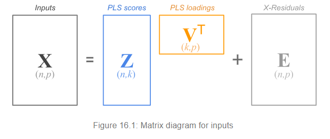
PLSR is another dimension reduction method to regularize a model, like PCR, PLSR seek subspace describe by ${\mathbf{z}}_1,...{\mathbf{z}}_{\mathbf{k}}$(or linear combinations of $\mathbf{X}$ )

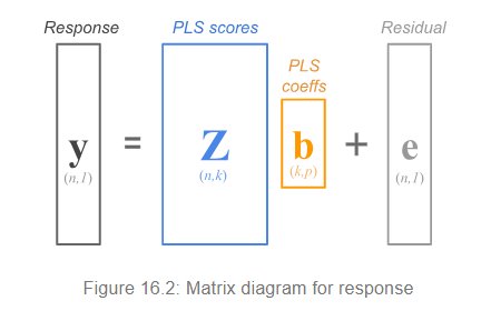
Moreover, there is an implicit assumption: $\mathbf{X}$ and $\mathbf{y}$ are assumed to be functions of a reduced $(k<p)$ number of components $\mathbf{Z}$ that can be used to decompose them

$$\mathbf{X}=\mathbf{Z}{\mathbf{V}}^{\mathsf{T}}+\mathbf{E}$$

$$\mathbf{y}=\mathbf{Z}\mathbf{b}+\mathbf{e}$$

So the model in the $X$-space is

$$\hat{\mathbf{X}}=\mathbf{Z}{\mathbf{V}}^{\mathrm{T}}$$

and y becomes

$$\hat{\mathbf{y}}=\mathbf{Z}\mathbf{b}$$

But How to get the components

Assume that both the inputs and the response are mean-centered(and possibly standardized). Compute the covariances between all the inputs variables and the reponse:

$${\tilde{\mathbf{w}}}_1=(cov({\mathbf{x}}_1,\mathbf{y}),\dots ,cov({\mathbf{x}}_p,\mathbf{y})).$$

In vector-matrix notation

$${\tilde{\mathbf{w}}}_1={\mathbf{X}}^{\mathrm{T}}\mathbf{y}$$

In fact, the notations above are not the same.
The matrix notation larger than the covariance
But we care about the direction only, and their direction will be the same if inputs and response are mean-centered(their mean is 0)
so it doesn’t matter

and we can also rescaled ${\tilde{\mathbf{w}}}_1$ by regressing each predictor ${\mathbf{x}}_{\mathbf{j}}$ onto $\mathbf{y}$

$${\tilde{\mathbf{w}}}_1={\mathbf{X}}^{\mathsf{T}}\mathbf{y}/{\mathbf{y}}^{\mathsf{T}}\mathbf{y}$$

and then normalize ${\tilde{\mathbf{w}}}_1$

$${\mathbf{w}}_1=\frac{{\tilde{\mathbf{w}}}_1}{||{\tilde{\mathbf{w}}}_1||}$$

We use these weights to compute the first component ${\mathbf{z}}_1$

$${\mathbf{z}}_1=w_{11}{\mathbf{x}}_1+...+w_{p1}{\mathbf{x}}_p$$

since ${\mathbf{w}}_1$ is unit-vector, the fomula can be expressed like

$${\mathbf{z}}_1=\mathbf{X}{\mathbf{w}}_1=\mathbf{X}{\mathbf{w}}_1/{\mathbf{w}}_1^{\mathsf{T}}{\mathbf{w}}_1$$

Then we use the component to regress inputs onto it to obtain the first PLS loading

$${\mathbf{v}}_1={\mathbf{X}}^{\mathsf{T}}{\mathbf{z}}_1/{\mathbf{z}}_1^{\mathsf{T}}{\mathbf{z}}_1$$

regress response onto it to obtain the first PLS coeffs

$$b_1={\mathbf{y}}^{\mathsf{T}}{\mathbf{z}}_1/{\mathbf{z}}_1^{\mathsf{T}}{\mathbf{z}}_1$$

And thus we have a first one-rank approximation

$$\hat{\mathbf{X}}={\mathbf{z}}_1{\mathbf{v}}_1^{\mathbf{T}}$$

Then we can obtain the rasidual matrix ${\mathbf{X}}_1$ (named deflation)

$${\mathbf{X}}_1=\mathbf{X}-\hat{\mathbf{X}}=\mathbf{X}-{\mathbf{z}}_1{\mathbf{v}}_1^{\mathsf{T}}(\mathrm{deflation})$$

deflate the response

$${\mathbf{y}}_1=\mathbf{y}-b_1{\mathbf{z}}_1$$

This is the first round, and we can obtain k components by repeating the process k times, iteratively

every time we reduce the rasidual by obtain the approximation of the previous rasidual matrix and the target $\mathbf{y}$
the effect of these approximation are synthesized by matrix multiply

个人认为，这么做的目的是通过回归的方式来拟合，得到降维子空间的同时减小产生的误差(每次都是拟合误差)，这些拟合的结果最终出现在矩阵中(开头的式子)，效果被综合

What PLS is doing is calculating all the different ingredients (e.g. ${\mathbf{w}}_{\mathbf{i}},{\mathbf{z}}_{\mathbf{i}},{\mathbf{v}}_{\mathbf{i}}$, $b_i$ ) separately, using least squares regressions. Hence the reason for its name partial least squares.

References

PCA

• Deep Learning - Foundations and Concepts
• Principal Component Analysis (PCA) Explained | Built In

PLSR

• 16 Partial Least Squares Regression | All Models Are Wrong: Concepts of Statistical Learning
• Partial least squares regression - Wikipedia

Difference

Not yet

• Principal Component Analysis (PCA) and Partial Least Squares (PLS) Technical Notes