Optimization Algorithm

How to choose an Optimization Algorithm

Optimization Algorithms

Optimization is a procedure for finding the parameters or arguments to a function that result in the minimum or maximum ouput.

The most common types in machine learning are continuous function optimization(连续函数优化)(real-valued numeric values 实数数值)

functions that take discrete variables are referred to as combinatorial optimization problems(组合优化问题)

Optimization algorithm can be grouped by the amount of information available about the target function
the more information that is available, the easier the function is to optimize

Perhaps the major division is whether the objective function canbe differentiated at a point or not (在某一点上是否能够微分)
or whether the first derivative (gradient or slope) of the function can be calculated for a given candidate solution or not.(是否能够计算一组解的导)
therefore Optimization algorithm can be divided to

• Algorithms that use derivative information
• Algorithms that do not use derivative information

Differentiable(可微的)

The first-order derivative(/dɪˈrɪv.ə.tɪv/) of a function is the rate or amount of change in the function at that point. It is often called the slope

the derivative of the function with multivariate inputs is referred to as the gradient
Gradient is a vector, and each element in the vector is called a partial derivative
partial derivative is the rate of change for a given variable at the point assuming all other variables are held constant(假设其他变量保持不变时的导)

The second-order derivative is the rate of change of the rate of change in the objective function.
For a function that takes multiple input variables, the second-order derivative is a matrix and is referred to as the Hessian matrix.

Optimization Algorithms that use the derivative

Bracketing Algorithms

Bracketing optimization algorithms are intended for optimization problems with one input variable where the optima is known to exist within a specific range.(一个变量，最优值在一个已知范围内)

some bracketing algorithms may be used without derivative information

Examples

• Fibonacci Search (斐波那契搜索)
• Golden Section Search (黄金分割法)
• Bisection Method (二分法)

Local Descent Algorithms

Local descent optimization algorithms are intended for optimization problems with more than one input variable and a single global optima (e.g. unimodal objective function 单峰目标函数). (多输入变量，单全局最优)

the most common example is the line search algorithm

• Line Search (线性搜索)

There are many variarions of the Line search
The procedure generally involves choosing a direction to move in the search space, then preforming a bracketing type search in a line or hyperplane(超平面) in the chosen direction
The limitation is that it is computationally expensive to optimize each directional move in the search space.

First-Order Algorithms

First-order optimization algorithms explicitly involve using the first derivative (gradient) to choose the direction to move in the search space.

The procedure involve first calculating the gradient, then following the gradient (in the opposite direction if in minimization problems) using a step size(learning rate).

the step size is a hyperparameter, deciding how far to move in the search space.
local descent algorithms perform a full line search for each directional move

A step size that is too small will takes a long time or even get stuck, whereas a step size that is too large will zig-zagging or bouncing around the search space, missing the optima

First-order algorithms are generally referred to as gradient descent.

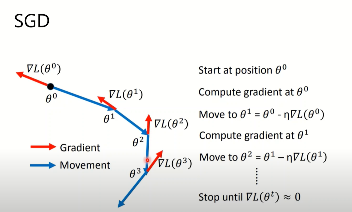
The gradient descent algorithm also provides the template for stochasitic(/stəˈkæs.tɪk/) version of the algorithm, named Stochastic Gradient Descent(SGD) (随机梯度下降)
The difference is that the gradient is appropriated rather than caculated directly(梯度不是直接计算出真实值而是估计的), using prediction error on traning data.

• Stochastic Gradient Descent (one sample)
• Batch Gradient Descent (all example)
• Mini-Batch Gradient Descent (subset of training data)

Second-Order Algorithms

Second-order optimization algorithms explicitly involve using the second derivative (Hessian) to choose the direction to move in the search space.

The algorithm are only used for objective function where Hessian matrix can be calculated or approximated.

For univariate objective function

• Newton’s Method
• Secant Method (割线法)

For multivariate objective function

• referred to as Quasi-Newton Method (拟牛顿法)
  • Davidson-Fletcher-Powell
  • Broyden-Fletcher-Goldfarb-Shanno (BFGS)
  • Limited-memory BFGS (L-BFGS)

Non-Differential Objective Function (非微分的)

There are functions where the derivative cannot be calculated, or the derivative can be calculated in some regions only, or is not a good guide.

The difficulties on objective functions

• No analytical description of the function (e.g. simulation)
• Multiple global optima (e.g. multimodal)
• Stochastic function evaluation (e.g. noisy)
• Discontinuous (e.g. regions with invalid soluns)

There are optimization algorithms that do not expect derivative information to be available.
These algorithms are referred to as black-box optimization algorithms as they assume little or nothing about objective function.

Direct Algorithms

Direct optimization algorithms are for objective functions for which derivatives cannot be calculated.

The algorithms are deterministic procedures(过程是确定性), and often assume the function has a single global optima.

Direct search are also typically referred to as a “pattern search”. They may navigate the search space using geometric shapes or decisions (patterns).

Gradient information is approximated directly from the result of the objective function comparing the relative difference between scores for points in the search space.
比较搜索空间中点的分数差来直接近似梯度信息，直接(direct)因此得名

These direct estimates are then used to choose a direction to move in the search space and triangulate the region of the optima.

Examples of direct search algorithms

• Cyclic Coordinate Search
• Powell’s Method
• Hooke-Jeeves Method
• Nelder-Mead Simplex Search

Stochastic Algorithms

Stochastic optimization algorithms are algorithms that make use of randomness in the search procedure for objective functions for which derivatives cannot be calculated.

stochastic algorithms typically involve a lot more sampling of the objective function, but are able to handle problems with deceptive local optima.

Include:

• Simulated Annealing (模拟退火)
• Evolution Strategy (演化策略)
• Cross-Entropy Method (交叉熵方法)

Population Algorithms

Population optimization algorithms(种群优化算法) are stochastic optimization algorithms that maintain a pool (a population) of candidate solutions that together are used to sample, explore, and hone in on an optima.
一组候选解(种群)，一起用于采样，探索，求最优解

Algorithms of this type are intended for more challenging objective problems that may have noisy function evaluations and many global optima (multimodal).
不得已之举

Examples

• Genetic Algorithm (遗传算法)
• Differential Evolution (差异进化算法)
• Particle Swarm Optimization (粒子群优化算法)

New optimization algorithm?

On-line learning: one pair of $(x_t,{\hat{y}}_t)$ at a time step
Off-line learning: all $(x_t,{\hat{y}}_t)$ at every time step
理论上训练需要所有的training data来进行计算loss，但是没有足够的资源(同时实做不见得所有数据是最优的)

假设每次都能计算所有的data

SGD(1847)

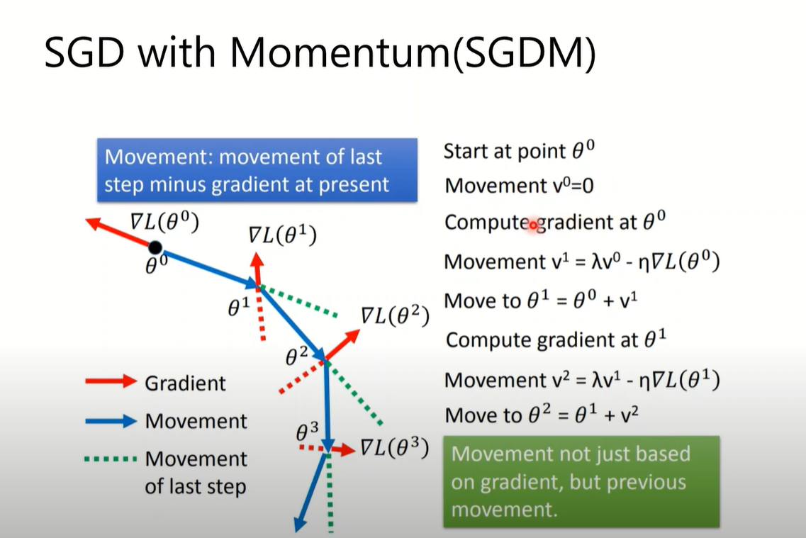
SGDM(Momentum)(1986)

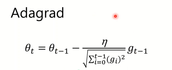
Adagrad(RMS+learning rate schedule)(2011)

$${\sigma }_i^t=\sqrt{\frac{1}{t+1}\sum _{j=0}^t(g_i^j{)}^2}$$ $${\eta }^t=\frac{\eta }{\sqrt{t+1}}$$ $$w^t=w^{t-1}-\frac{\eta }{\sqrt{{\sum }_{j=0}^{t+1}(g^j{)}^2}}{g}^{t-1}$$

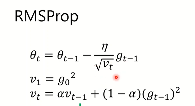
RMSProp(Exponential moving average/EMA)(2013)
调节新梯度的权重

Adam(2015)

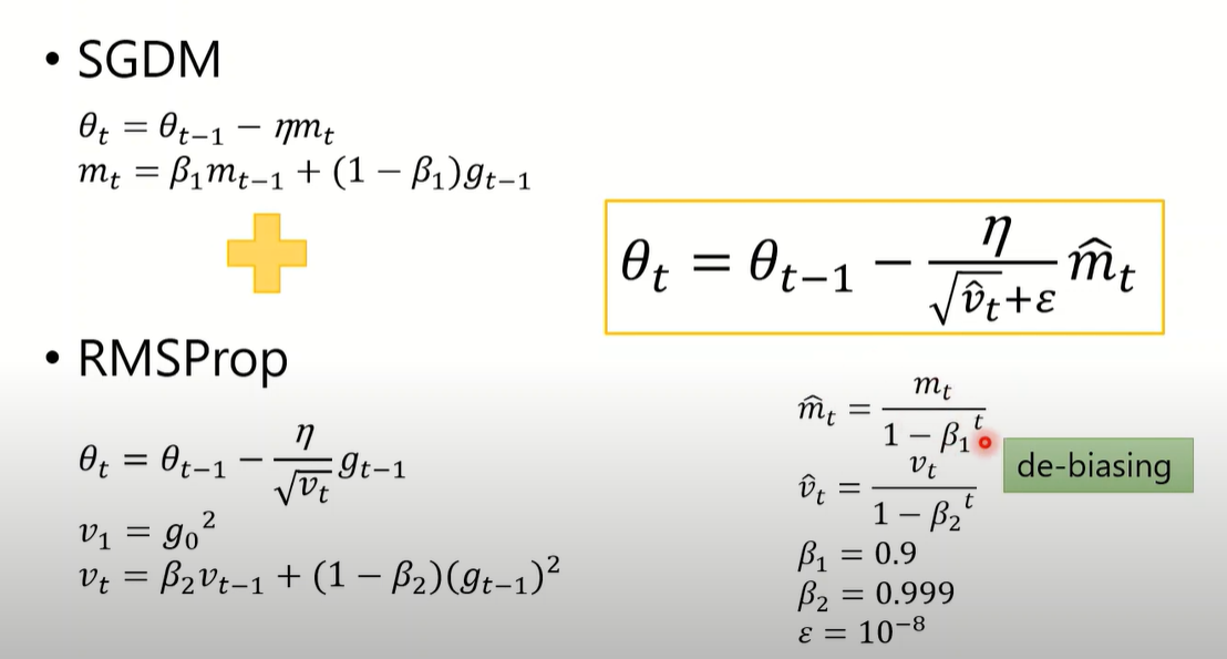
SGDM+RMSProp，但是movement的计算方式改为了EMA，同时对$m$ 和 $v$进行了调整

Adam vs SGDM

SGD，SGDM固定learning rate
Adagrad，RMSProp，Adam adaptive learning rate
从实际来看，Adam和SGDM表现最好

Adam: fast training, large generalization gap(validation 落差大), unstable
SGDM: stable, little generalization gap, better convergence

Combine Adam with SGDM?

什么时候切换，切换时需要什么原则
大概还没解决

有个SWATS算法

Improving Adam

实际训练的时候，会产生很多没有指导性的gradient，虽然很小但是综合起来会产生较大的影响

AMSGrad(2018)

减小non-informative gradients的影响，去掉de-biasing

• 原本$v$的计算会不断加入新的梯度，历史的梯度不断乘以小数，历史的占比会逐渐消失，存在记忆的时间长度
• 如果前面有一个有指向性的梯度(大的梯度)，它对学习率的影响会随着时间消失
• 则non-informative的梯度产生的影响会变大。
• AMSGrad取前一次计算和当前v中的最大值，实际上是在比较梯度平方和历史梯度加权和的大小，保留大的那个以保留历史

但是这样的话，会使得v逐渐变大，可能导致训练不起来，实际上也不见得，只是不太完善

AdaBound(2019)

AMSGrad 是处理当梯度很小时learning rate太大的情况，也需要处理梯度很大时learning rate太小的情况

• 限定上下界

Improving SGDM

没有learning rate的调整，训练比较慢
由LR range test得到learning rate适中时表现比较好

Cyclical LR(2017)

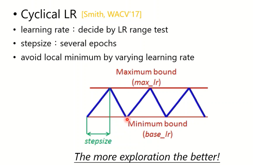
• max和base值是由LR range test 决定
• stepsize 几个epochs

SGDR(2017)

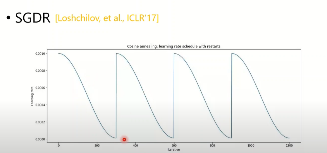
• 直接从头开始，没有逐渐变大的过程

One-cycle LR(2017)

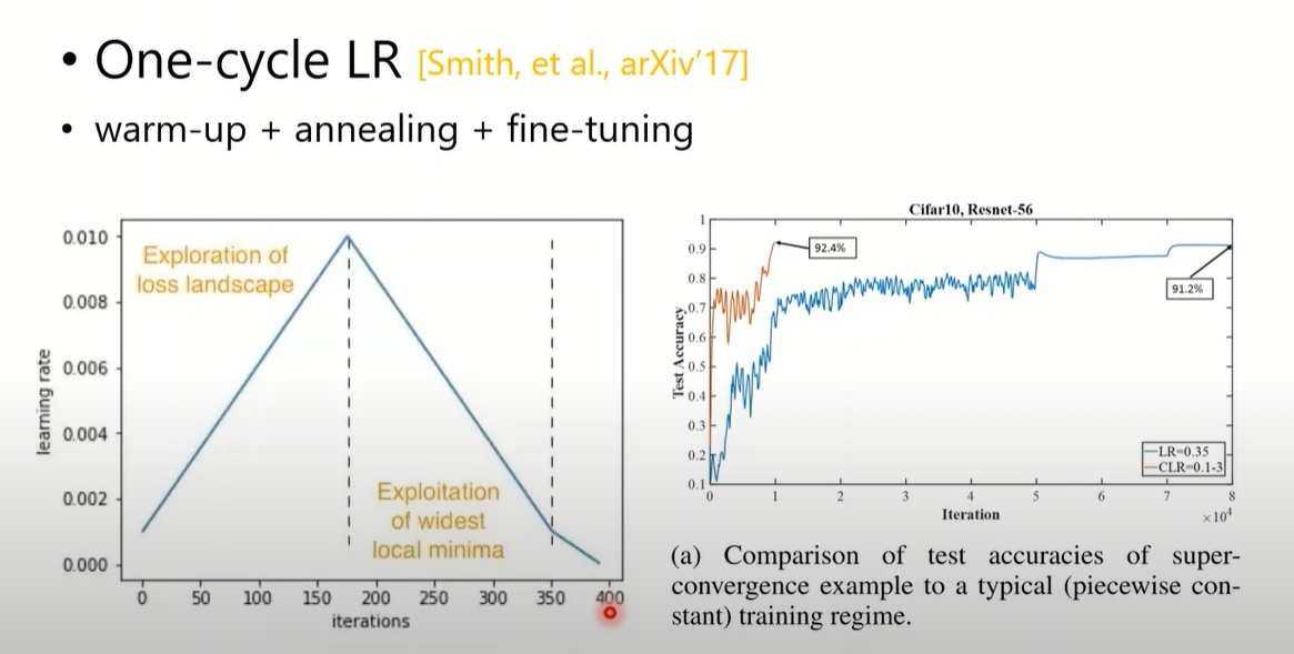
• 只有一个cycle，加上一个微调

Adam and warm-up

weight initialization 的时候，可能会导致初始的梯度很乱，此时adaptive learning rate 获取的信息不足，调整不稳定，实验表明warm-up能缓解这件事。
所以Adam可能需要warm-up
一般是Linear increase (几千步)。

RAdam(2020)

非直线，而是计算warm-up learning rate

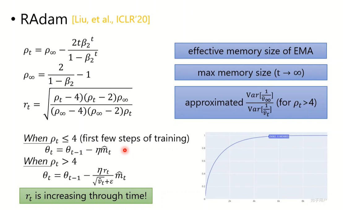
• $\rho$ 的计算是为了计算 $r$,，$r$的计算是为了估计$\frac{var(1/{\hat{v}}_{\infty })}{var(1/{\hat{v}}_t)}$，之所以结果和梯度无关是因为假设梯度遵循Gaussian
• $r$的估计在${\rho }_t\le 4$ 时，估计并不准确，前几轮先用SGDM
• 当$\hat{v}$ 方差越大时，代表此时梯度变化越乱，学习率应当减小以削弱影响
• $r$的变化曲线如右下角，随时间逼近1

Look the future

Lookahead(2019)

universal wrapper for all optimizers
通用的优化器的附件？
k step forward, 1 step back

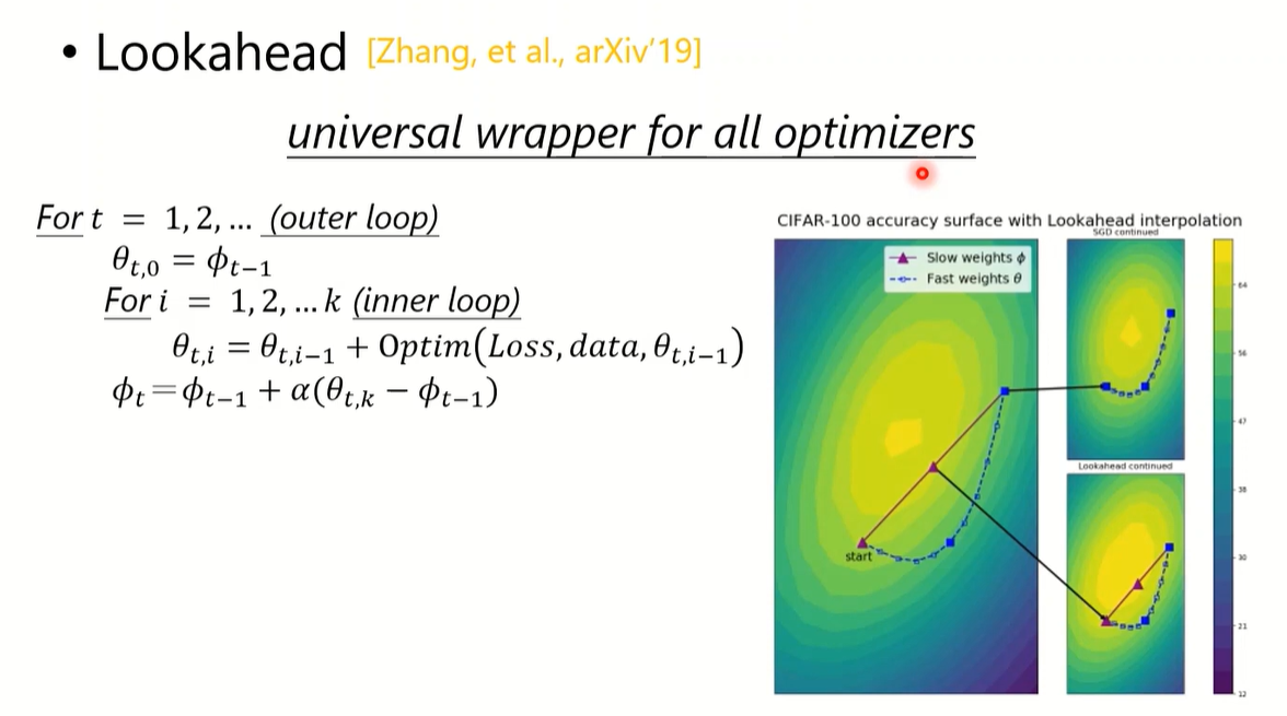
• 两组weight，$\varphi$ slow weight，$\theta$ fast weight
• fast weight 先更新几步，然后slow weight取更新结果的中间某一个点，进行下次迭代
• fast weight做exploration，slow weight进行实际的更新

更稳定，同时有利于寻找平坦的最小值

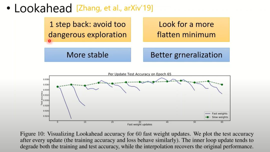
• 如果是危险的exploration可以撤回 — more stable
• 如果是崎岖的minimum会减少进入的可能 — better generalization

Nesterov accelerated gradient(NAG) (1983)

look into the future

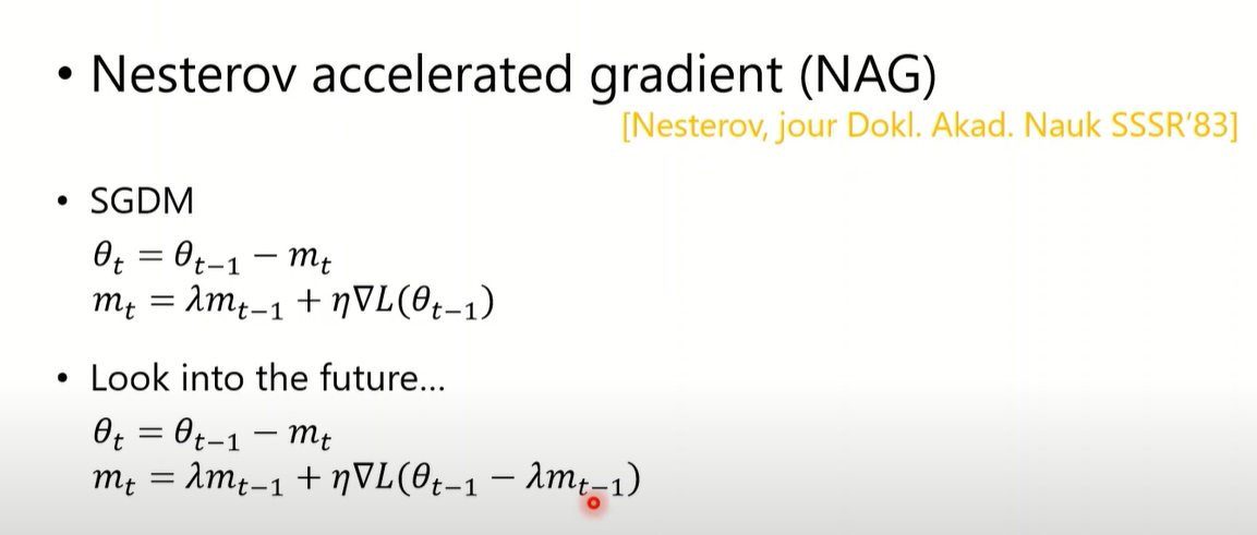
• 这里的符号做了修改，正负改变，结果等价
• 修改momentum计算，加上一个特殊点的梯度，估计未来的情况
• ${\theta }_{t-1}-\lambda m_{t-1}$ 是用过去数据估计未来可能到达的点

目前这样得维护当前参数的值，一份更新一份计算未来梯度
可以通过数学推导简化过程(也没有很简化)

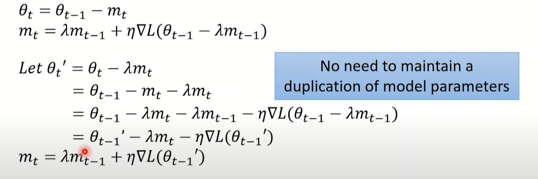
• 维护${\theta }^{\prime }$，movement的更新由当前的$\theta ’$ 得到
• 新${\theta }^{\prime }$ 通过当前$\theta ’$ 和 movement计算得到，不需要再对当前参数进行两次更改

另一个角度
NAG中参数更新为

SGDM中参数更新为

可以写成

则NAG可以看成，尽管参数不同，但是将movement改成了未来的情况$m_{t-1}\to m_t$

Nadam(2016)

Adam + NAG
计算$m_t$ 的de-biasing可以拆成

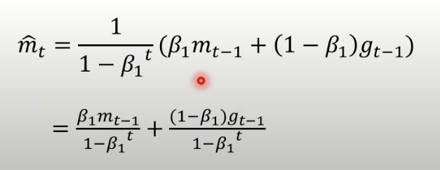
然后改一下$m_{t-1}$

About L2 regularization

由于momentum $m$ 和adaptive learning rate $v$ 的计算都涉及到Loss function，那该不该让$m,v$ 的计算受到L2 regularization的影响

AdamW & SGDWM

只对权重的更新进行L2正则化，而$m,v$正常计算
只有weight decay

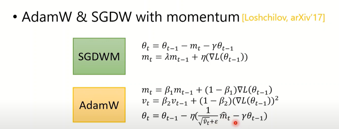
这个算法比较有用
AdamW 用于BERT

Others

Exploration

Encourage exploration

• shuffling 随机分batch
• Gropout
• Gradient noise
  • 
  • 加一个Gaussian noise，随时间减小

During learning

• Warm-up

• Curriculum learning

  • 
  • 先用简单数据训练，再使用困难数据

• Fine-tuning

  • pre-trained model

• Normalization

• Regularization

Summary

SGDM v.s. Adam

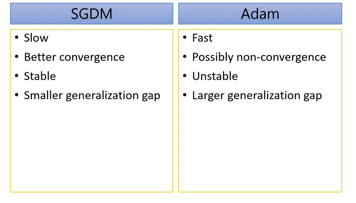
Advice

• SGDM
  • CV
• Adam
  • NLP
  • GAN
  • RL (大概)

References

• How to Choose an Optimization Algorithm
• torch.optim — PyTorch 2.4 documentation
• [TA 補充課] Optimization for Deep Learning (1/2) (由助教簡仲明同學講授) - YouTube
• [TA 補充課] Optimization for Deep Learning (2/2) (由助教簡仲明同學講授) - YouTube