Flow Matching

README & Reference

README

主要是英文记录（大多是抄的），然后如果很难表达或者理解比较困难会切换成中文

真的要看以下内容务必结合reference原文

Reference

[2506.02070] An Introduction to Flow Matching and Diffusion Models 👍

非常好课程，非常好材料

Flow and Diffusion Models

Flow Models

Introduction

We modeling the reverse process by ordinary differential equations(ODEs).
Generally, A solution to an ODE is defined by a trajectory

$$X:[0,1]\to {\mathbb{R}}^d,t\mapsto X_t,$$

$X$ is a function that map time t to some location in space $R^d$ (d维向量)

The formulation of ODE is

$$\frac{\mathrm{d}}{\mathrm{d}t}{X}_t=f(X_t)$$

rewrite $f(X_t)$ as $u_t(X_t)$. In perspective of physics, $u_t(X_t)$ is called vector field and define an ODE.

$$u:{\mathbb{R}}^d\times [0,1]\to {\mathbb{R}}^d,(x,t)\mapsto u_t(x),$$

It is we need an ODE that its trajectory X follows along the lines of vector field $u_t$
And the trajectory should also strat from point $x_0$

$$\begin{array}{rl}\frac{\mathrm{d}}{\mathrm{d}t}{X}_t& =u_t(X_t)\\ X_0& =x_0\end{array}$$

Given the ODE and vector field above, we can solve the ODE and obtain its solution. The solution is called flow

$$\begin{array}{rl}\psi :{\mathbb{R}}^d\times [0,1]& \mapsto {\mathbb{R}}^d,(x_0,t)\mapsto {\psi }_t(x_0)\\ \frac{\mathrm{d}}{\mathrm{d}t}{\psi }_t(x_0)& =u_t({\psi }_t(x_0))\\ {\psi }_0(x_0)& =x_0\end{array}$$

given a timestep t and the original location $x_0$. flow $\psi$ recover the trajectory $X_t$

In a word, we define ODE by vector field and its solution is flow

Theorem 1 Flow existence and uniqueness
If $u:{\mathbb{R}}^d\times [0,1]\to {\mathbb{R}}^d$ is continuously differentiable with a bounded derivative, then the ODE has a unique solution given by a flow ${\psi }_t.$ In this case, ${\psi }_t$is a diffeomorpism(微分同构) for all $t$, ($\text{ i.e. }{\psi }_t$ is continuously differentiable with a continuously differentiable inverse ${\psi }_t^{-1}.$)

The neural networks are always bounded derivative, so we can assume that all the ODE discussed has unique solution(flow)

Simulating ODE

It is difficult to compute flow $\psi ()$ explicitly if $u$ is not as simple as a linear function
We could use numerical methods instead

One of the simplest and most intuitive methods is Euler method

$$X_{t+h}=X_t+h{u}_t(X_t)(t=0,h,2h,3h,\dots ,1-h)$$

Where $h$ is the timestep gap

A more complicated method: Heun’s method

$$\begin{array}{rl}{X}_{t+h}^{\prime }& =X_t+h{u}_t(X_t)▶\text{ initial guess of new state}\\ X_{t+h}& =X_t+\frac{h}{2}(u_t(X_t)+u_{t+h}(X_{t+h}^{\prime }))▶\text{ update with average }u\text{ at current and guessed state}\end{array}$$

Heun method take a initial step to get a guess state, and correct the direction via an updated step

We can define the flow model
Given an ODE:

$$\begin{array}{rl}{X}_0& \sim p_{\text{init}}▶\text{ random initialization}\\ \frac{\text{d}}{\text{d}t}{X}_t& =u_t^{\theta }(X_t)▶\text{ ODE}\end{array}$$

flow model paramterizes the vector field $u^{\theta }$, and with ODE solver we can obtain the trajectory, and thus reach the target distribution
Actually, we do not care about what the trajectory looks like. We just want a efficient and high-quality path(defined by vector field) to map source distribution to target distribution. So flow models learn vector field instead of flow

Not that precise

By now, we only talk about the sample process(we have obtained the ODE)(trajectory→vector field→ODE)
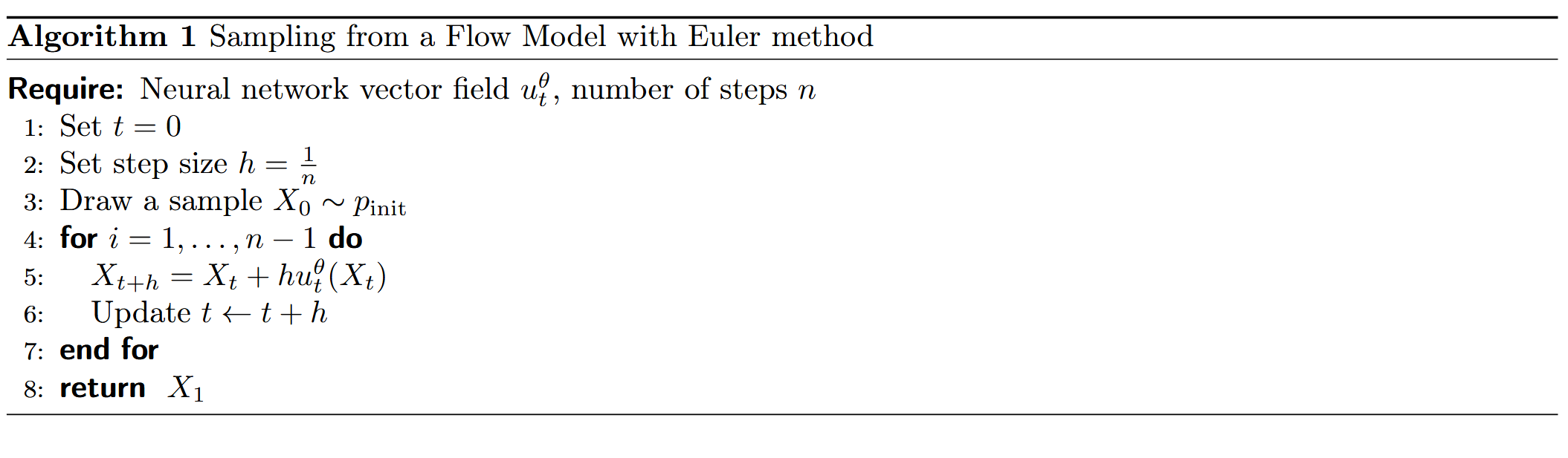
The Pseudo-algorithm can be writen as

Diffuision Models

Stochastic differential equations(SDEs) extend the ODE with stochastic trajectories. A stochastic trajectory is called a stochastic process
The stochastic process is given by

$$\begin{array}{r}{X}_t\text{ is a random variable for every }0\le t\le 1\\ X:[0,1]\to {\mathbb{R}}^d,t\mapsto X_t\text{ is a random trajectory for every draw of }X\end{array}$$

Simulate stochastic process twice, we might get different outcomes

Brownian Motion

A Brownian motion $W=(W_t{)}_{0\le t\le 1}$ is a stochastic process such that $W_0=0$
The brownian motion define a stochastic trajectories $t\mapsto W_t$, the trajectories are continuous and the following conditions are hold

• Normal increments:
  • $W_t-W_s\sim \mathcal{N}(0,(t-s)I_d)$ for all $0\le s<t$
  • Increments have a Gaussian distribution with variance increasing linearly in time ($I_d$ is the identity matrix)
• Independent increments:
  • for $0\le t_0<t<...<t_n=1$, the increments $W_{t_1}-W_{t_0},...W_{t_n}-W_{t_{n-1}}$ are independent random variables

Brownian motion is also called Wiener process. We can easily simulate a Brownian motion approximately with step size $h>0$ by setting $W_0=0$ and updating $W_{t+h}=W_t+\sqrt{h}{ϵ}_t,{ϵ}_t\sim \mathcal{N}(0,I_d)(t=0,h,2h,...1-h)$

From ODEs to SDEs

Then we try to transform ODEs to SDEs by adding brownian motion
Since brownian is totally stochastic(continuous but indifferentiable), we need a equivalent formulation of ODEs that does not use derivatives

$$\begin{array}{rl}\frac{d}{dt}{X}_t& =u_t(X_t)\\ \stackrel{(i)}{⟺}\frac{1}{h}(X_{t+h}-X_t)& =u_t(X_t)+R_t(h)\\ \iff X_{t+h}& =X_t+h{u}_t(X_t)+h{R}_t(h)\end{array}$$

We use a differential form instead, where $R_t(h)$ is a negligible error function/term
Then we add brownian motion

$$X_{t+h}=X_t+\underset{\text{deterministic}}{\underbrace{h{u}_t(X_t)}}+\underset{\text{stochastic}}{\underbrace{{\sigma }_t(W_{t+h}-W_t)}}+\underset{\text{error term}}{\underbrace{h{R}_t(h)}}$$

$\sigma$ describes the diffusion coefficient and $R_t(h)$ describes a stochastic error term. ( $\mathbb{E}[||R_t(h)|{|}^2{]}^{1/2}\to 0$ for $h\to 0$ ). This equation is called stochastic differential equation. It can be denoted as

$$\begin{array}{rl}d{X}_t& =u_t(X_t)dt+{\sigma }_{t}d{W}_t\\ X_0& =x_0\end{array}$$

keep in mind that $dX$ notation is informal

SDEs always don’t have analytical solution, so we need a numerical method(like Euler method in ODE). The corresponding method is Euler-Maruyama method.
It can be write in a general form

$$X(t+h)\approx X(t)+u_t(X_t)h+{\sigma }_{t}d{W}_t$$

Or

$$X_{t+h}=X_t+h{u}_t(X_t)+\sqrt{h}{\sigma }_t{ϵ}_t,{ϵ}_t\sim \mathcal{N}(0,I_d)$$

The tutorial use $h$ for denote $\Delta t$, the term $\sqrt{h}{\sigma }_t{ϵ}_t$ here may be easier to understand by denoted as ${\sigma }_t{ϵ}_t\sqrt{\Delta t}$. where $\sigma$ is the coefficient and $ϵ$ is a Gaussian noise
One may ask why $\sqrt{\Delta t}$ here?
An easy answer of the question would be: the variance of brownian motion is $t$, so that $\sqrt{t}$ is its std. For $\Delta W$, std becomes $\sqrt{\Delta t}$. We need a Gaussian distribution which has variance $\Delta t$, so we multiply $\sqrt{\Delta t}$ here.

Diffusion Models

diffusion model aims to model SDE, a simple way is to parameterize also the vector field.

$$\begin{array}{rl}\mathrm{d}{X}_t=u_t^{\theta }(X_t)\mathrm{d}t+{\sigma }_t\mathrm{d}{W}_t& ▶\text{ SDE}\\ X_0\sim p_{\text{init}}& ▶\text{ random initialization}\end{array}$$

This is still a sample process: initialize a $X_0$ from simple distribution, simulate the SDE from 0 to 1, and obtain the goal $X_1$

Constructing the Training Target

We have learned about how to sample via vector field, which is parameterized by network. To train a neural network that perform as the actual vector field, we need to find a training target

$$\mathcal{L}(\theta )=\Vert u_t^{\theta }(x)-\underset{\text{training target}}{\underbrace{u_t^{\text{target}}(x)}}{\Vert }^2,$$

target should itself be a vector field that converts $p_{init}$ into $p_{data}$. But if we can directly obtain that target vector field, using neural network and train a alternative is just waste of time.
We can’t find the exact vector field, but we can derive a process that have the same performance: converts $p_{init}$ into $p_{data}$

Conditional and Marginal Probability Path

A probability path is specifis a gradual interpolation between two distribution

Given noise $p_{init}$ and data $p_{data}$, let’s say, the data point belong to Dirac delta “distribution” $\delta$, which means that samling from $\delta$, the results are always the same (deterministic)

Given data point $z$, the Dirac delta distribution is ${\delta }_z$, always return $z$

The conditional(interpolating) probability path is a set of distribution $p_t(x|z)$ such that:

$$p_0(\cdot |z)=p_{\text{init}},p_1(\cdot |z)={\delta }_z\text{for all }z\in {\mathbb{R}}^d.$$

in the axes of time step, $p_t(x|z)$ is the conditional probability path, but given a time step $t$, $p_t(x|z)$ is the conditional ditribution

A conditional probability path gradually converts a single data point into the distribution $p_{init}$. Every conditional probability path $p_t(x|z)$ induces a marginal probability path $p_t(x)$

we know how to sample from $p_t$, but we don’t know the density values as the integral is intractable

$$\begin{array}{rl}z\sim p_{\text{data}},x\sim p_t(\cdot |z)⟹x\sim p_t& ▶\text{ sampling from marginal path}\\ p_t(x)=\int p_t(x|z)p_{\text{data}}(z)\mathrm{d}z& ▶\text{ density of marginal path}\end{array}$$

we can only sample from the distribution/path and we can not compute the $p_t(x)$ from a specific $x$

In practice, we always define a simple conditional path as long as they fullfill the requirements: $p_0(\cdot |z)=p_{\text{init}},p_1(\cdot |z)={\delta }_z\text{for all }z\in {\mathbb{R}}^d.$

like Gaussain conditional path

$$p_t(\cdot |z)=\mathcal{N}({\alpha }_{t}z,{\beta }_t^2{I}_d)▶\text{ Gaussian conditional path}$$ $$z\sim p_{\text{data}},ϵ\sim p_{\text{init}}=\mathcal{N}(0,I_d)⟹x={\alpha }_{t}z+{\beta }_tϵ\sim p_t▶\text{ sampling from marginal Gaussian path}$$

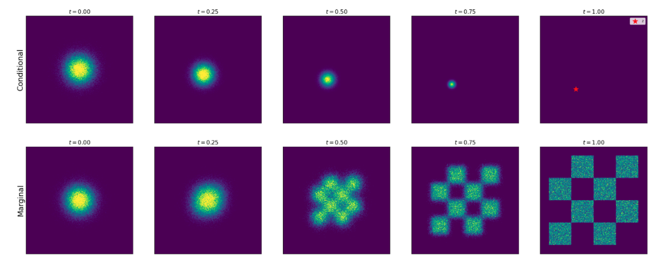
这里展示的是conditional path和marginal path的区别，实际上是基础数学理解的问题，conditonal path是一个给定 data point z 和 具体的path 形式之后得到的 随时间的分布，可视化中是具体的某个图像的去噪/加噪过程，可视化中是具体图像的原因，是作为随机性的部分（噪声可视化中每个时刻已经被确定） marginal path即使给定了具体的path形式，整体仍然是分布，这里的toy demo是将这个分布做成了棋牌桌的样子 所以这里是 固定某个数据样本， 和整个数据集之间的区别

Conditional and Marginal Vector Fields

Theorem 10

Based on the notations mentioned above, we can derive the target vector field:
$u_t^{\text{target}}(\cdot |z)$ denote a conditional vector field
defined so that the corresponding ODE yields the conditional probability path $p_t(\cdot |z)$ :

$$X_0\sim p_{\text{init}},\frac{\mathrm{d}}{\mathrm{d}t}{X}_t=u_t^{\text{target}}(X_t|z)⟹X_t\sim p_t(\cdot |z)(0\le t\le 1).$$

the marginal vector field defined by

$$u_t^{\text{target}}(x)=\int u_t^{\text{target}}(x|z)\frac{p_t(x|z)p_{\text{data}}(z)}{p_t(x)}\mathrm{d}z,$$

the mariginal probability path:

$$X_0\sim p_{\text{init}},\frac{\mathrm{d}}{\mathrm{d}t}{X}_t=u_t^{\text{target}}(X_t)⟹X_t\sim p_t(0\le t\le 1).$$

Why it useful

before prove it, we first figure out why it useful:
The article said, construct the marginal vector field from a conditional vector field simplifies the the problem of finding a formula for a training target significantly

we can find a conditional vector field and derive the target vector field
It can be illustrated by the Gaussain example

let $p_t(\cdot |z)=\mathcal{N}({\alpha }_{t}z,{\beta }_t^2{I}_d)$
define conditional flow

$${\psi }_t^{\text{target}}(x|z)={\alpha }_{t}z+{\beta }_{t}x.$$

Given $X_0$ satisfy $X_0\sim \mathcal{N}(0,I_d)$

$$X_t={\psi }_t^{\text{target}}(X_0|z)={\alpha }_{t}z+{\beta }_t{X}_0\sim \mathcal{N}({\alpha }_{t}z,{\beta }^2{I}_d)=p_t(\cdot |z).$$

Remember that flow is the solution of a ODE, and vector field define a ODE
We found a conditional vector field that satisfy theorem 10

$$\begin{array}{rl}\frac{\mathrm{d}}{\mathrm{d}t}{\psi }_t^{\text{target}}(x|z)& =u_t^{\text{target}}({\psi }_t^{\text{target}}(x|z)|z)\text{for all }x,z\in {\mathbb{R}}^d\\ \stackrel{(i)}{\iff }{\dot{\alpha }}_{t}z+{\dot{\beta }}_{t}x& =u_t^{\text{target}}({\alpha }_{t}z+{\beta }_{t}x|z)\text{for all }x,z\in {\mathbb{R}}^d\\ \stackrel{(ii)}{\iff }{\dot{\alpha }}_{t}z+{\dot{\beta }}_t\left(\frac{x-{\alpha }_{t}z}{{\beta }_t}\right)& =u_t^{\text{target}}(x|z)\text{for all }x,z\in {\mathbb{R}}^d\\ \stackrel{(iii)}{\iff }\left({\dot{\alpha }}_t-\frac{{\dot{\beta }}_t}{{\beta }_t}{\alpha }_t\right)z+\frac{{\dot{\beta }}_t}{{\beta }_t}x& =u_t^{\text{target}}(x|z)\text{for all }x,z\in {\mathbb{R}}^d\end{array}$$

How to prove it

切换中文解释比较复杂的内容 theorem 10 can be proved via the continuity equation

define divergence operator div

$$\text{div}(v_t)(x)=\sum _{i=1}^d\frac{\partial }{\partial x_i}{v}_t(x)$$

continuity equation:

$${\partial }_t{p}_t(x)=-\text{div}(p_t{u}_t^{\text{target}})(x)\text{for all }x\in {\mathbb{R}}^d,0\le t\le 1,$$

这里的连续性方程可以被理解为： 左边是概率密度随时间的变化，右边是x位置净流入率（散度在物理中经常描述净流出率） 对于左边而言，计算单纯是对这个位置计算随时间t的密度变化，那么自然会等于 密度乘以速度得到质量之后的对位置的导数

只要vector field满足连续性方程，根据某个定理就可以证明这个vector field就是我们想要的target vector field（充要条件），所以给定定理10前提(对应ii转化)，可以得到以下推导证明定理10

$$\begin{array}{rl}{\partial }_t{p}_t(x)& \stackrel{(i)}{=}{\partial }_t\int p_t(x|z)p_{\text{data}}(z)\mathrm{d}z\\ & =\int {\partial }_t{p}_t(x|z)p_{\text{data}}(z)\mathrm{d}z\\ & \stackrel{(ii)}{=}\int -\text{div}(p_t(\cdot |z)u_t^{\text{target}}(\cdot |z))(x)p_{\text{data}}(z)\mathrm{d}z\\ & \stackrel{(iii)}{=}-\text{div}\left(\int p_t(x|z)u_t^{\text{target}}(x|z)p_{\text{data}}(z)\mathrm{d}z\right)\\ & \stackrel{(iv)}{=}-\text{div}\left(p_t(x)\int u_t^{\text{target}}(x|z)\frac{p_t(x|z)p_{\text{data}}(z)}{p_t(x)}\mathrm{d}z\right)(x)\\ & \stackrel{(v)}{=}-\text{div}\left(p_t{u}_t^{\text{target}}\right)(x),\end{array}$$

Conditional and Marginal Score Functions

Now we extend the reasoning to SDEs

define the marginal score function of $p_t$ as $\nabla \log p_t(x)$

remember that SDE is denoted as

$$\begin{array}{rl}d{X}_t& =u_t(X_t)dt+{\sigma }_{t}d{W}_t\\ X_0& =x_0\end{array}$$

Theorem 13

for diffusion coefficient ${\sigma }_t\ge 0$ , we can construct an SDE which follows the same probability path:

$$\begin{array}{rl}{X}_0\sim p_{\text{init}},\mathrm{d}{X}_t& =\left[u_t^{\text{target}}(X_t)+\frac{{\sigma }_t^2}{2}\nabla \log p_t(X_t)\right]\mathrm{d}t+{\sigma }_t\mathrm{d}{W}_t\\ ⟹X_t\sim p_t& (0\le t\le 1)\end{array}$$

the same identity holds if we change marginal expression to conditional expression

Similar to before, the theorem 13 is useful because it is way more easier to find a conditional score function.

$$\nabla \log p_t(x)=\frac{\nabla p_t(x)}{p_t(x)}=\frac{\nabla \int p_t(x|z)p_{\text{data}}(z)\mathrm{d}z}{p_t(x)}=\frac{\int \nabla p_t(x|z)p_{\text{data}}(z)\mathrm{d}z}{p_t(x)}=\int \nabla \log p_t(x|z)\frac{p_t(x|z)p_{\text{data}}(z)}{p_t(x)}\mathrm{d}z$$

How to prove it

依旧切换中文

定理13可以通过Fokker-Planck equation证明，首先同样定义一个特殊算子

Laplacian operator

$$\Delta w_t(x)=\sum _{i=1}^d\frac{{\partial }^2}{{\partial }^2{x}_i}{w}_t(x)=\text{div}(\nabla w_t)(x).$$

有定理15（Fokker-Planck Equation）
给定一个SDE

$$X_0\sim p_{\text{init}},\mathrm{d}{X}_t=u_t(X_t)\mathrm{d}t+{\sigma }_t\mathrm{d}{W}_t.$$

$X_t$ 属于分布 $p_t$ 当且仅当满足Fokker-Planck equation

$${\partial }_t{p}_t(x)=-\text{div}(p_t{u}_t)(x)+\frac{{\sigma }_t^2}{2}\Delta p_t(x)\text{for all }x\in {\mathbb{R}}^d,0\le t\le 1.$$

Fokker-Planck equation比较复杂，没有太直觉的解释，直接将定理13的前提代入可以得到

$$\begin{array}{rl}{\partial }_t{p}_t(x)& \stackrel{(i)}{=}-\text{div}(p_t{u}_t^{\text{target}})(x)\\ & \stackrel{(ii)}{=}-\text{div}(p_t{u}_t^{\text{target}})(x)-\frac{{\sigma }_t^2}{2}\Delta p_t(x)+\frac{{\sigma }_t^2}{2}\Delta p_t(x)\\ & \stackrel{(iii)}{=}-\text{div}(p_t{u}_t^{\text{target}})(x)-\text{div}\left(\frac{{\sigma }_t^2}{2}\nabla p_t\right)(x)+\frac{{\sigma }_t^2}{2}\Delta p_t(x)\\ & \stackrel{(iv)}{=}-\text{div}(p_t{u}_t^{\text{target}})(x)-\text{div}\left(p_t\left[\frac{{\sigma }_t^2}{2}\nabla \log p_t\right]\right)(x)+\frac{{\sigma }_t^2}{2}\Delta p_t(x)\\ & \stackrel{(v)}{=}-\text{div}\left(p_t\left[u_t^{\text{target}}+\frac{{\sigma }_t^2}{2}\nabla \log p_t\right]\right)(x)+\frac{{\sigma }_t^2}{2}\Delta p_t(x),\end{array}$$

iv和v用到了div算子的特殊性质（log和线性计算）

Langevin dynamics

if the probability path is static, i.e. $p_t=p$ for a fixed distribution $p$
vector field should be 0 and the SDE is

$$\mathrm{d}{X}_t=\frac{{\sigma }_t^2}{2}\nabla \log p(X_t)\mathrm{d}t+{\sigma }_t\mathrm{d}{W}_t,$$

this is known as Langevin dynamics

Langevin dynamics有一些特性
因为p固定，p是这个Langevin dynamics的稳定分布

• $X_0\sim p⟹X_t\sim p$
• $X_0\sim p^{\prime }$ 且 $p^{\prime }\ne p$时，随着演化，最终也会得到分布 p

Training the Generative Model

Flow Matching

since we have derive target vector field, we can use MSE loss for training

$$\begin{array}{rl}{\mathcal{L}}_{\text{FM}}(\theta )& ={\mathbb{E}}_{t\sim \text{Unif},x\sim p_t}[\Vert u_t^{\theta }(x)-u_t^{\text{target}}(x){\Vert }^2]\\ & \stackrel{(i)}{=}{\mathbb{E}}_{t\sim \text{Unif},z\sim p_{\text{data}},x\sim p_t(\cdot |z)}[\Vert u_t^{\theta }(x)-u_t^{\text{target}}(x){\Vert }^2],\end{array}$$

The loss means that we first sample timestep, and then sample a data point z, and compute x (sample from $p_t(\cdot |z)$)

$$u_t^{\text{target}}(x)=\int u_t^{\text{target}}(x|z)\frac{p_t(x|z)p_{\text{data}}(z)}{p_t(x)}\mathrm{d}z,$$

But the integral is intractable, we cannot directly compute the value of target vector field. Instead we using conditonal flow matching loss

$${\mathcal{L}}_{\text{CFM}}(\theta )={\mathbb{E}}_{t\sim \text{Unif},z\sim p_{\text{data}},x\sim p_t(\cdot |z)}[\Vert u_t^{\theta }(x)-u_t^{\text{target}}(x|z){\Vert }^2].$$

Training on conditional vector field makes no sense if we only care about marginal vector field unless they are the same

Theorem 18

The marginal flow matching loss equals the conditional flow matching loss up to a constant

$${\mathcal{L}}_{\text{FM}}(\theta )={\mathcal{L}}_{\text{CFM}}(\theta )+C,$$

so that their gradient are the same

$${\nabla }_{\theta }{\mathcal{L}}_{\text{FM}}(\theta )={\nabla }_{\theta }{\mathcal{L}}_{\text{CFM}}(\theta ).$$

Proof:

$$\begin{array}{rl}{\mathcal{L}}_{\mathrm{FM}}(\theta )& \stackrel{(i)}{=}{\mathbb{E}}_{t\sim \mathrm{Unif},x\sim p_t}[\Vert u_t^{\theta }(x)-u_t^{\mathrm{target}}(x){\Vert }^2]\\ & \stackrel{(ii)}{=}{\mathbb{E}}_{t\sim \mathrm{Unif},x\sim p_t}[\Vert u_t^{\theta }(x){\Vert }^2-2u_t^{\theta }(x{)}^T{u}_t^{\mathrm{target}}(x)+\Vert u_t^{\mathrm{target}}(x){\Vert }^2]\\ & \stackrel{(iii)}{=}{\mathbb{E}}_{t\sim \mathrm{Unif},x\sim p_t}[\Vert u_t^{\theta }(x){\Vert }^2]-2{\mathbb{E}}_{t\sim \mathrm{Unif},x\sim p_t}[u_t^{\theta }(x{)}^T{u}_t^{\mathrm{target}}(x)]+\underset{=:C_1}{\underbrace{{\mathbb{E}}_{t\sim \mathrm{Unif}[0,1],x\sim p_t}[\Vert u_t^{\mathrm{target}}(x){\Vert }^2]}}\\ & \stackrel{(iv)}{=}{\mathbb{E}}_{t\sim \mathrm{Unif},z\sim p_{\mathrm{data}},x\sim p_t(\cdot |z)}[\Vert u_t^{\theta }(x){\Vert }^2]-2{\mathbb{E}}_{t\sim \mathrm{Unif},x\sim p_t}[u_t^{\theta }(x{)}^T{u}_t^{\mathrm{target}}(x)]+C_1\end{array}$$

the second summand is

$$\begin{array}{rl}{\mathbb{E}}_{t\sim \mathrm{Unif},x\sim p_t}[u_t^{\theta }(x{)}^T{u}_t^{\mathrm{target}}(x)]& \stackrel{(i)}{=}{\int }_0^1\int p_t(x)u_t^{\theta }(x{)}^T{u}_t^{\mathrm{target}}(x)\mathrm{d}x\mathrm{d}t\\ & \stackrel{(ii)}{=}{\int }_0^1\int p_t(x)u_t^{\theta }(x{)}^T\left[\int u_t^{\mathrm{target}}(x|z)\frac{p_t(x|z)p_{\mathrm{data}}(z)}{p_t(x)}\mathrm{d}z\right]\mathrm{d}x\mathrm{d}t\\ & \stackrel{(iii)}{=}{\int }_0^1\int \int u_t^{\theta }(x{)}^T{u}_t^{\mathrm{target}}(x|z)p_t(x|z)p_{\mathrm{data}}(z)\mathrm{d}z\mathrm{d}x\mathrm{d}t\\ & \stackrel{(iv)}{=}{\mathbb{E}}_{t\sim \mathrm{Unif},z\sim p_{\mathrm{data}},x\sim p_t(\cdot |z)}[u_t^{\theta }(x{)}^T{u}_t^{\mathrm{target}}(x|z)]\end{array}$$

It means that, using the same derivation, CFM can be convey by a same first summand, a same second summand and a constan, sothat we proof the theorem 18

$$\begin{array}{rl}{\mathcal{L}}_{\mathrm{FM}}(\theta )& \stackrel{(i)}{=}{\mathbb{E}}_{t\sim \mathrm{Unif},z\sim p_{\mathrm{data}},x\sim p_t(\cdot |z)}[\Vert u_t^{\theta }(x){\Vert }^2]-2{\mathbb{E}}_{t\sim \mathrm{Unif},z\sim p_{\mathrm{data}},x\sim p_t(\cdot |z)}[u_t^{\theta }(x{)}^T{u}_t^{\mathrm{target}}(x|z)]+C_1\\ & \stackrel{(ii)}{=}{\mathbb{E}}_{t\sim \mathrm{Unif},z\sim p_{\mathrm{data}},x\sim p_t(\cdot |z)}[\Vert u_t^{\theta }(x){\Vert }^2-2u_t^{\theta }(x{)}^T{u}_t^{\mathrm{target}}(x|z)+\Vert u_t^{\mathrm{target}}(x|z){\Vert }^2-\Vert u_t^{\mathrm{target}}(x|z){\Vert }^2]+C_1\\ & \stackrel{(iii)}{=}{\mathbb{E}}_{t\sim \mathrm{Unif},z\sim p_{\mathrm{data}},x\sim p_t(\cdot |z)}[\Vert u_t^{\theta }(x)-u_t^{\mathrm{target}}(x|z){\Vert }^2]+\underset{=:C_2}{\underbrace{{\mathbb{E}}_{t\sim \mathrm{Unif},z\sim p_{\mathrm{data}},x\sim p_t(\cdot |z)}[-\Vert u_t^{\mathrm{target}}(x|z){\Vert }^2]}}+C_1\\ & \stackrel{(iv)}{=}{\mathcal{L}}_{\mathrm{CFM}}(\theta )+\underset{=:C}{\underbrace{C_2+C_1}}\end{array}$$

Score Matching

The SDE if defined by

$$\begin{array}{rl}\mathrm{d}{X}_t& =\left[u_t^{\text{target}}(X_t)+\frac{{\sigma }_t^2}{2}\nabla \log p_t(X_t)\right]\mathrm{d}t+{\sigma }_t\mathrm{d}{W}_t\\ X_0& \sim p_{\text{init}},\\ ⟹X_t& \sim p_t(0\le t\le 1)\end{array}$$

loss can be desined as

$$\begin{array}{rl}{\mathcal{L}}_{\text{SM}}(\theta )={\mathbb{E}}_{t\sim \text{Unif},z\sim p_{\text{data}},x\sim p_t(\cdot |z)}[\Vert s_t^{\theta }(x)-\nabla \log p_t(x){\Vert }^2]& ▶\text{ score matching loss}\\ {\mathcal{L}}_{\text{CSM}}(\theta )={\mathbb{E}}_{t\sim \text{Unif},z\sim p_{\text{data}},x\sim p_t(\cdot |z)}[\Vert s_t^{\theta }(x)-\nabla \log p_t(x|z){\Vert }^2]& ▶\text{ conditional score matching loss}\end{array}$$

And similarily, conditional score function is available objective for score matching.

$$\nabla \log p_t(x)=\int \nabla \log p_t(x|z)\frac{p_t(x|z)p_{\text{data}}(z)}{p_t(x)}\mathrm{d}z.$$

marginal score function looks the same as marginal vector field and therefore they has the same theorem and proof

Theorem 20

$${\mathcal{L}}_{\text{SM}}(\theta )={\mathcal{L}}_{\text{CSM}}(\theta )+C,$$ $${\nabla }_{\theta }{\mathcal{L}}_{\text{SM}}(\theta )={\nabla }_{\theta }{\mathcal{L}}_{\text{CSM}}(\theta ).$$

Gaussian example

ODE 的Gaussian example没有什么好说的，需要再回来看就行，SDE实际上需要训练两个模型，分别拟合 vector field 和 score function

如果真的这么做了，一方面比较麻烦（两个模型或者两个输出），另一方面有些误差存在（当然flow matching和score matching都有误差）

对于score matching来说，生成结果受模型精度影响，它有随机噪声 $\sigma$，这个$\sigma$的数值会很大影响结果，可以作为误差的调整，也可能导致误差变大

对于Gaussian的例子，实际上不需要训练两个模型或者两个head

对于Gaussain的例子，首先conditional score function是

$$\nabla \log p_t(x|z)=-\frac{x-{\alpha }_{t}z}{{\beta }_t^2}.$$ $$\begin{array}{rl}{\mathcal{L}}_{\text{CSM}}(\theta )& ={\mathbb{E}}_{t\sim \text{Unif},z\sim p_{\text{data}},x\sim p_t(\cdot |z)}[\Vert s_t^{\theta }(x)+\frac{x-{\alpha }_{t}z}{{\beta }_t^2}{\Vert }^2]\\ & \stackrel{(i)}{=}{\mathbb{E}}_{t\sim \text{Unif},z\sim p_{\text{data}},ϵ\sim \mathcal{N}(0,I_d)}[\Vert s_t^{\theta }({\alpha }_{t}z+{\beta }_tϵ)+\frac{ϵ}{{\beta }_t}{\Vert }^2]\\ & ={\mathbb{E}}_{t\sim \text{Unif},z\sim p_{\text{data}},ϵ\sim \mathcal{N}(0,I_d)}\left[\frac{1}{{\beta }_t^2}\Vert {\beta }_t{s}_t^{\theta }({\alpha }_{t}z+{\beta }_tϵ)+ϵ{\Vert }^2\right]\end{array}$$

这个损失也叫 denoising score matching

但是这里如果 $\beta$ 接近0的话，数值不稳定
DDPM中是直接去掉 $\frac{1}{{\beta }^2}$，同时把 $s_t^{\theta }$ 改成noise predictor network ${ϵ}_t^{\theta }$

$$-{\beta }_t{s}_t^{\theta }(x)={ϵ}_t^{\theta }(x)⟹{\mathcal{L}}_{\text{DDPM}}(\theta )={\mathbb{E}}_{t\sim \text{Unif},z\sim p_{\text{data}},ϵ\sim \mathcal{N}(0,I_d)}[\Vert {ϵ}_t^{\theta }({\alpha }_{t}z+{\beta }_tϵ)-ϵ{\Vert }^2]$$

除此之外，Gaussian除了能够直接得到conditional score function之外，score funciton 和 vector field 可以相互转化

设$p_t(x|z)=\mathcal{N}({\alpha }_{t}z,{\beta }_t^2{I}_d)$
有

$$u_t^{\text{target}}(x|z)=\left({\beta }_t^2\frac{{\dot{\alpha }}_t}{{\alpha }_t}-{\dot{\beta }}_t{\beta }_t\right)\nabla \log p_t(x|z)+\frac{{\dot{\alpha }}_t}{{\alpha }_t}x$$ $$u_t^{\text{target}}(x)=\left({\beta }_t^2\frac{{\dot{\alpha }}_t}{{\alpha }_t}-{\dot{\beta }}_t{\beta }_t\right)\nabla \log p_t(x)+\frac{{\dot{\alpha }}_t}{{\alpha }_t}x$$

marginal vector对应得这个ODE称为 probability flow ODE

证明为

$$u_t^{\text{target}}(x|z)=\left({\dot{\alpha }}_t-\frac{{\dot{\beta }}_t}{{\beta }_t}{\alpha }_t\right)z+\frac{{\dot{\beta }}_t}{{\beta }_t}x\stackrel{(i)}{=}\left({\beta }_t^2\frac{{\dot{\alpha }}_t}{{\alpha }_t}-{\dot{\beta }}_t{\beta }_t\right)\left(\frac{{\alpha }_{t}z-x}{{\beta }_t^2}\right)+\frac{{\dot{\alpha }}_t}{{\alpha }_t}x=\left({\beta }_t^2\frac{{\dot{\alpha }}_t}{{\alpha }_t}-{\dot{\beta }}_t{\beta }_t\right)\nabla \log p_t(x|z)+\frac{{\dot{\alpha }}_t}{{\alpha }_t}x$$

i就是从式子中凑出score function

代入marginal flow vector的积分可以直接得到另一个式子

$$\begin{array}{rl}{u}_t^{\text{target}}(x)& =\int u_t^{\text{target}}(x|z)\frac{p_t(x|z)p_{\text{data}}(z)}{p_t(x)}\mathrm{d}z=\int \left[\left({\beta }_t^2\frac{{\dot{\alpha }}_t}{{\alpha }_t}-{\dot{\beta }}_t{\beta }_t\right)\nabla \log p_t(x|z)+\frac{{\dot{\alpha }}_t}{{\alpha }_t}x\right]\frac{p_t(x|z)p_{\text{data}}(z)}{p_t(x)}\mathrm{d}z\\ & \stackrel{(i)}{=}\left({\beta }_t^2\frac{{\dot{\alpha }}_t}{{\alpha }_t}-{\dot{\beta }}_t{\beta }_t\right)\nabla \log p_t(x)+\frac{{\dot{\alpha }}_t}{{\alpha }_t}x\end{array}$$

如果通过vector field计算score function的话

$$u_t^{\theta }=\left({\beta }_t^2\frac{{\dot{\alpha }}_t}{{\alpha }_t}-{\dot{\beta }}_t{\beta }_t\right)s_t^{\theta }(x)+\frac{{\dot{\alpha }}_t}{{\alpha }_t}x.$$ $$s_t^{\theta }(x)=\frac{{\alpha }_t{u}_t^{\theta }(x)-{\dot{\alpha }}_{t}x}{{\beta }_t^2{\dot{\alpha }}_t-{\alpha }_t{\dot{\beta }}_t{\beta }_t}.$$

因此，denoising score matching 和 conditional flow matching 是一致的（也就是在Gaussian probability path下两个损失等价）
如果训练denoising score matching之后希望通过SDE进行采样

$$X_0\sim p_{\text{init}},\mathrm{d}{X}_t=\left[\left({\beta }_t^2\frac{{\dot{\alpha }}_t}{{\alpha }_t}-{\dot{\beta }}_t{\beta }_t+\frac{{\sigma }_t^2}{2}\right)s_t^{\theta }(x)+\frac{{\dot{\alpha }}_t}{{\alpha }_t}x\right]\mathrm{d}t+{\sigma }_t\mathrm{d}{W}_t$$

A Guide to the Diffusion Model Literature

• Discrete time and continuous time
  • Discrete time came from the early diffusion paper. Using discrete time should choose a time discretization before training. The loss function is approximated via an evidence lower bound(ELBO), which is only a lower bound of the loss.
  • Song showed that actually discrete constructions were essentially an approximation of a time-continuous SDEs and the ELBO loss is the tight loss in continuous case
• Forward process & probability paths
  • probability path in this document means a set of ditribution that satisfy $p_0=p_{init},p_1=p_{data}$. it indicate a trajectory between noise and data point, but in term of ditribution across time.
  • early diffusion use forward process to describe this process, add noise to the data point, and for $T\gg 0$, ${\bar{X}}_T\sim \mathcal{N}(0,I_d)$
  • The difference is: forward process describe a specific path in probability path (how to convert a data point into noise), but probability path is more general and do not care how to convert data.
  • In practice, we need to know the distribution of $X_t|X_0=z$ in closed form in order to train our models to avoid simulating the SDE. vector field in forward process are always of the affine form $u_t(x)=a_{t}x$ where $a_t$ is a continuous function
• Time-Reversals & Solving the Fokker-Planck equation
  • early diffusion model use time reversals (reverse the forward process) to derive the training objective. But we do not care about how to obtain data point (through time reversal), we just care about $X_1\sim p_{data}$. A true reversal is not necessary
• Flow Matching and Stochastic Interpolants
  • The framework that we present is most closely related to the frameworks of flow matching and stochastic interpolants (SIs)
  • Stochastic interpolants included both the pure flow and the SDE extension via “Langevin dynamics”

文中提到了Flow Matching 的框架下，不需要定义forward过程（随时间的变化过程），只需要定义概率路径（init和data之间的中间随机变量$X_t$ ），求解ODE的过程是确定性，不依赖于随机过程
大概的意思应该是 之前的diffusion或者SDE的做法，需要构建复杂的前向和反向过程，对于FM来说，可以直接定义简单的概率路径，例如线性插值，直接得到速度场得到target，同时是scalable的

Summary

方便理解使用中文
有点一知半解，梳理一下概念

• Flow Matching 和 Score Matching都是训练方法，根据probability flow ODE，训练结果都可以用于SDE或者ODE的求解
• probability flow ODE和SDE拥有相同边缘概率分布，但是probability flow ODE是ODE，给定初始点轨迹确定，SDE给定初始点仍然存在随机过程，二者轨迹不同
• flow model 和 diffusion model分别对应了ODE建模和SDE建模

实际上还差一些相关工作，不过需要的时候再回来进一步梳理吧